knitr::opts_chunk$set(echo = TRUE)
# Necessary Packages
library(tidyverse)
library(ggplot2)
library(fastDummies)
library(rworldmap)
library(lubridate)

City of New York Shooting Data

For this project, I decided to focus my analysis on answering the question: Have shootings and murders decreased over time in New York? I think there are a lot of different ways to slice the data and investigate both the overall result, as well as population specific results.

This data is provided directly from the City of New York City. The data itself comes from the New York Police Department (NYPD) and will record one row per shooting incident.

Import & Read Data

Importing directly from the site.

url_in <- "https://data.cityofnewyork.us/api/views/833y-fsy8/rows.csv"

shooting <- read_csv(url_in)

Tidying Data

# Removing coordinates
shooting1 <- shooting %>% select(-c(X_COORD_CD, Y_COORD_CD))

# Mutating dates, additional columns
shooting1 <- shooting1 %>% mutate(DATE_TIME = as.POSIXct(paste(OCCUR_DATE," ",OCCUR_TIME),format = "%m/%d/%Y  %H:%M:%S")) %>% mutate(SAME_AGE_GROUP = case_when(PERP_AGE_GROUP == VIC_AGE_GROUP ~ 1, TRUE ~ 0)) %>% mutate(SAME_SEX = case_when(PERP_SEX == VIC_SEX ~ 1, TRUE ~ 0)) %>% mutate(SAME_RACE = case_when(PERP_RACE == VIC_RACE ~ 1, TRUE ~ 0)) %>% mutate(MURDER = case_when(STATISTICAL_MURDER_FLAG == TRUE ~ 1, TRUE ~ 0)) %>% 
  mutate(YEAR = year(DATE_TIME), MONTH = month(DATE_TIME), WEEK_DAY = wday(DATE_TIME))

# Dummy columns for categorical data
shooting2 <- dummy_cols(shooting1, select_columns = c('PERP_AGE_GROUP', 'PERP_SEX', 'PERP_RACE', 'VIC_AGE_GROUP', 'VIC_SEX', 'VIC_RACE'), remove_selected_columns = FALSE)

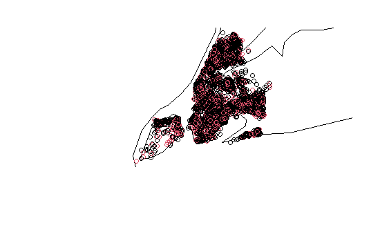
Mapping Incidents (for fun!)

nyc_map <- getMap(resolution = 'low')
nyc_map_plot <- plot(nyc_map, xlim= c(min(shooting2$Longitude),max(shooting2$Longitude)), ylim= c(min(shooting2$Latitude),max(shooting2$Latitude))) + points(shooting2$Longitude, shooting2$Latitude, col= factor(shooting2$MURDER))

Analyzing Data

# Summarizing shootings by year and borough
shootings_year_b <- shooting2 %>% group_by(YEAR, BORO) %>% summarize (
  total = n(), 
  murders = sum(MURDER, na.rm=T), 
  perp_m = sum(PERP_SEX_M, na.rm=T), 
  perp_f = sum(PERP_SEX_F, na.rm=T), 
  vic_m = sum(VIC_SEX_M, na.rm=T),
  vic_f = sum(VIC_SEX_F, na.rm=T)
)

# Adding in percent columns
shootings_year_b <- shootings_year_b %>% mutate(pct_murder = murders/total, pct_perp_m = perp_m/total, pct_perp_f = perp_f/total, pct_vic_m = vic_m/total, pct_vic_f = vic_f/total)

shootings_year_b

YEAR	BORO	total	murders	perp_m	perp_f	vic_m	vic_f	pct_murder	pct_perp_m
2006	BRONX	568	137	450	9	511	57	0.24119718	0.7922535
2006	BROOKLYN	850	176	637	4	784	66	0.20705882	0.7494118
2006	MANHATTAN	288	60	213	4	262	26	0.20833333	0.7395833
2006	QUEENS	296	59	229	3	276	20	0.19932432	0.7736486
2006	STATEN ISLAND	53	13	45	2	40	13	0.24528302	0.8490566
2007	BRONX	533	93	425	9	486	46	0.17448405	0.7973734
2007	BROOKLYN	833	177	586	13	765	67	0.21248499	0.7034814
2007	MANHATTAN	233	46	182	3	217	14	0.19742489	0.7811159
2007	QUEENS	238	48	162	5	210	28	0.20168067	0.6806723
2007	STATEN ISLAND	50	9	43	2	43	7	0.18000000	0.8600000

Note: this is a subset of the full table results.

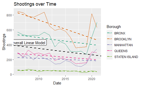
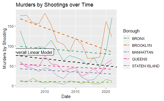
2006 in Brooklyn had the most overall shootings (by borough and year) at 850. The top 7 results by total shooting are all Brooklyn (2006, 2011, 2007, 2020, 2010, 2008, 2009). By murders, Brooklyn takes the top 3 spots (2010, 2007, and 2006 respectfully), but the fourth highest is the Bronx in 2021. In contrast, the lowest amount of shootings was Staten Island in 2006.

Modeling

mod_shootings <- lm(total ~ YEAR, data = shootings_year_b)
mod_murders <- lm(murders ~ YEAR, data = shootings_year_b)
mod_pct_murders <- lm(pct_murder ~ YEAR, data = shootings_year_b)

summary(mod_shootings)$coefficients[,1]
summary(mod_murders)$coefficients[,1]
summary(mod_pct_murders)$coefficients[,1]

 (Intercept)         YEAR 
17838.584412    -8.700588 
(Intercept)        YEAR 
3588.778235   -1.751765 
  (Intercept)          YEAR 
-0.5638202432  0.0003760115 

Plots

ggplot(shootings_year_b) +
  geom_line(mapping=aes(x = YEAR, y = total, color = BORO)) +
  labs(x="Date", y="Shootings", title="Shootings over Time", color = "Borough") +
  scale_color_brewer(palette="Dark2") +
  geom_smooth(mapping=aes(x = YEAR, y = total, color = BORO), method = "lm", se=F, linetype=2) +
  geom_abline(mapping=aes(intercept=summary(mod_shootings)$coefficients[1],slope=summary(mod_shootings)$coefficients[2]), col = 'black', linetype = 2, size=1) +
  geom_label(aes(2008,430, label='Overall Linear Model'))

ggplot(shootings_year_b) +
  geom_line(mapping=aes(YEAR, murders, color = BORO)) +
  labs(x="Date", y="Murders by Shooting", title="Murders by Shootings over Time", color = "Borough") +
  scale_color_brewer(palette="Dark2") +
  geom_smooth(mapping=aes(x = YEAR, y = murders, color = BORO), method = "lm", se=F, linetype=2) + 
  geom_abline(mapping=aes(intercept=summary(mod_murders)$coefficients[1],slope=summary(mod_murders)$coefficients[2]), col = 'black', linetype = 2, size=1) +
  geom_label(aes(2008,85, label='Overall Linear Model'))

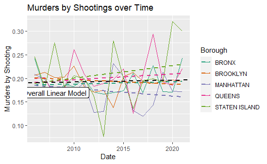
ggplot(shootings_year_b) +
  geom_line(mapping=aes(YEAR, pct_murder, color = BORO)) +
  labs(x="Date", y="Murders by Shooting", title="Murders by Shootings over Time", color = "Borough") +
  scale_color_brewer(palette="Dark2") +
  geom_smooth(mapping=aes(x = YEAR, y = pct_murder, color = BORO), method = "lm", se=F, linetype=2) + 
  geom_abline(mapping=aes(intercept=summary(mod_pct_murders)$coefficients[1],slope=summary(mod_pct_murders)$coefficients[2]), col = 'black', linetype = 2, size=1) +
  geom_label(aes(2008,.17, label='Overall Linear Model'))

Reflections and Potential Bias

From the plots above, one can conclude that shootings and murders have decreased over time; however, there were notable spikes in 2020, which is especially concerning given 2020 was the start of the global COVID-19 pandemic. Even more interesting, while both have decreased, the percent of shootings that are murders have not decreased, and if anything, are slightly increasing overall.

This leads to more questions on the ratios, or percent, of shootings and shooting murders that other populations are experiences. One could easily replicate parts of this analysis to investigate age, race, and sex related metrics to see if the total and rate of shootings are increasing or decreasing.

One important bias to point out is that this data is in total people. I decided not to find and join borough specific population data over time, so we cannot infer anything about the rate of shootings or shooting murders in a specific borough. This data may also hold the same implicit-biases that the NYPD, and potentially police forces in general have. Similarly, the data may not reflect ‘all’ shooting instances, as it is likely that not all shootings are reported to police.