Purpose

This project is to help me learn python syntax and packages and familiarize myself with the ecosystem as a whole. I tried to use various techniques for describing and mutating data, as well as displaying data.

Unfortunately, I could not get my plotly plots to load correctly, so click here for a PDF of the plotly graphs.

import pandas as pd
import numpy as np
import matplotlib as mpl
import matplotlib.pyplot as plt
import plotly as pl
import plotly.express as px
import scipy as sp
import scipy.stats
from sklearn.linear_model import LinearRegression

plt.style.use("classic")
%matplotlib inline

Loading in Data

netflix_raw = pd.read_csv('Netflix Dataset Latest 2021.csv')

Filtering Data to Relevant Columns

netflix_1 = netflix_raw[['Title',
 'Genre',
 'Tags',
 'Languages',
 'Series or Movie',
 'Country Availability',
 'Runtime',
 'IMDb Score',
 'Rotten Tomatoes Score',
 'Metacritic Score',
 'Awards Received',
 'Awards Nominated For',
 'Boxoffice',
 'Release Date',
 'Netflix Release Date']].copy()

netflix_1 = netflix_1.astype("int64", errors="ignore")
netflix_1 = netflix_1.astype({"Title": "string",
 'Genre': "string",
 'Tags': "string",
 'Languages': "string",
 'Series or Movie': "string",
 'Country Availability': "string",
 'Boxoffice': "float"}, errors='ignore')
netflix_1["Release Date"] = pd.to_datetime(netflix_1["Release Date"])
netflix_1["Netflix Release Date"] = pd.to_datetime(netflix_1["Netflix Release Date"])
netflix_1["Same Day Rel"] = (netflix_1["Release Date"] == netflix_1["Netflix Release Date"])
netflix_1["USA Availability"] = netflix_1["Country Availability"].str.contains(pat = "United States")

Creating New DataTables for analysis

netflix_rel = netflix_1.loc[netflix_1["Same Day Rel"] == True]
netflix_nonrel = netflix_1.loc[netflix_1["Same Day Rel"] == False]

netflix_series = netflix_1.loc[netflix_1["Series or Movie"] == "Series"]
netflix_movie = netflix_1.loc[netflix_1["Series or Movie"] == "Movie"]

netflix_usa = netflix_1.loc[netflix_1["USA Availability"] == True]
netflix_int = netflix_1.loc[netflix_1["USA Availability"] == False]

We will be trying to research the following questions:

Are same day Netflix releases better or worse than non-same day release titles?
Are Netflix Movies or Series better?
Are Netflix offerings in the US better than international offerings?

Are same day Netflix releases better or worse than non-same day release titles?

Using the netflix_rel and netflix_nonrel tables, we will try to answer if there is any difference on the quality of same day releases vs. non-same day releases. We can assume same day release title are Netflix exclusives or titles that worked closely with Netflix to produce, as Netflix has not historically partnered with studios to release new titles the same day as theaters.

I will use numpy functionality to find values and matplotlib to plot histograms.

rel_imdb = np.array(netflix_rel["IMDb Score"])
rel_rt = np.array(netflix_rel["Rotten Tomatoes Score"])
rel_mc = np.array(netflix_rel["Metacritic Score"])
rel_awards_n = np.array(netflix_rel["Awards Nominated For"])
rel_awards_r = np.array(netflix_rel["Awards Received"])

nonrel_imdb = np.array(netflix_nonrel["IMDb Score"])
nonrel_rt = np.array(netflix_nonrel["Rotten Tomatoes Score"])
nonrel_mc = np.array(netflix_nonrel["Metacritic Score"])
nonrel_awards_n = np.array(netflix_nonrel["Awards Nominated For"])
nonrel_awards_r = np.array(netflix_nonrel["Awards Received"])

v_rel_imdb = np.array([np.nanmean(rel_imdb), np.nanmedian(rel_imdb), np.nanmin(rel_imdb), np.nanmax(rel_imdb)])
v_rel_rt = np.array([np.nanmean(rel_rt), np.nanmedian(rel_rt), np.nanmin(rel_rt), np.nanmax(rel_rt)])
v_rel_mc = np.array([np.nanmean(rel_mc), np.nanmedian(rel_mc), np.nanmin(rel_mc), np.nanmax(rel_mc)])
v_rel_awards_n = np.array([np.nanmean(rel_awards_n), np.nanmedian(rel_awards_n), np.nanmin(rel_awards_n), np.nanmax(rel_awards_n)])
v_rel_awards_r = np.array([np.nanmean(rel_awards_r), np.nanmedian(rel_awards_r), np.nanmin(rel_awards_r), np.nanmax(rel_awards_r)])

v_nonrel_imdb = np.array([np.nanmean(nonrel_imdb), np.nanmedian(nonrel_imdb), np.nanmin(nonrel_imdb), np.nanmax(nonrel_imdb)])
v_nonrel_rt = np.array([np.nanmean(nonrel_rt), np.nanmedian(nonrel_rt), np.nanmin(nonrel_rt), np.nanmax(nonrel_rt)])
v_nonrel_mc = np.array([np.nanmean(nonrel_mc), np.nanmedian(nonrel_mc), np.nanmin(nonrel_mc), np.nanmax(nonrel_mc)])
v_nonrel_awards_n = np.array([np.nanmean(nonrel_awards_n), np.nanmedian(nonrel_awards_n), np.nanmin(nonrel_awards_n), np.nanmax(nonrel_awards_n)])
v_nonrel_awards_r = np.array([np.nanmean(nonrel_awards_r), np.nanmedian(nonrel_awards_r), np.nanmin(nonrel_awards_r), np.nanmax(nonrel_awards_r)])

print(np.vstack([v_rel_imdb,v_nonrel_imdb,(v_rel_imdb - v_nonrel_imdb)]))

print(np.vstack([v_rel_rt,v_nonrel_rt,(v_rel_rt - v_nonrel_rt)]))

print(np.vstack([v_rel_mc,v_nonrel_mc,(v_rel_mc - v_nonrel_mc)]))

print(np.vstack([v_rel_awards_n,v_nonrel_awards_n,(v_rel_awards_n - v_nonrel_awards_n)]))

print(np.vstack([v_rel_awards_r,v_nonrel_awards_r,(v_rel_awards_r - v_nonrel_awards_r)]))

    [[ 7.08104313  7.1         3.1         9.3       ]
     [ 6.94065321  7.          1.6         9.7       ]
     [ 0.14038992  0.1         1.5        -0.4       ]]
    [[ 74.69407895  81.           0.         100.        ]
     [ 64.09978603  69.           0.         100.        ]
     [ 10.59429291  12.           0.           0.        ]]
    [[ 62.64609053  65.          18.          94.        ]
     [ 57.82651732  58.           6.         100.        ]
     [  4.81957321   7.          12.          -6.        ]]
    [[ 10.58964143   4.           1.         334.        ]
     [ 16.50102145   6.           1.         386.        ]
     [ -5.91138002  -2.           0.         -52.        ]]
    [[   5.95166163    3.            1.          127.        ]
     [   9.9918284     4.            1.          300.        ]
     [  -4.04016676   -1.            0.         -173.        ]]

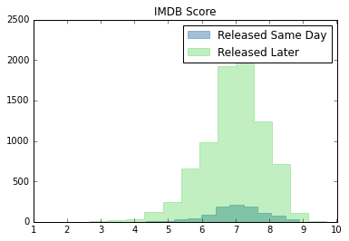
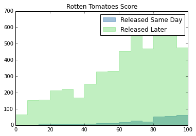
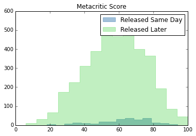
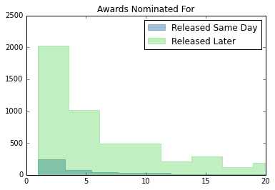
Matplotlib Histogram Plots

plt.hist(netflix_rel["IMDb Score"], bins=15, histtype="stepfilled", color="steelblue", edgecolor="steelblue", alpha = 0.5, label="Released Same Day")
plt.hist(netflix_nonrel["IMDb Score"], bins=15, histtype="stepfilled", color="limegreen", edgecolor="limegreen", alpha = 0.3,  label="Released Later")
plt.legend()
plt.title("IMDB Score")

    Text(0.5, 1.0, 'IMDB Score')

png

plt.hist(netflix_rel["Rotten Tomatoes Score"], bins=15, histtype="stepfilled", color="steelblue", edgecolor="steelblue", alpha = 0.5, label="Released Same Day")
plt.hist(netflix_nonrel["Rotten Tomatoes Score"], bins=15, histtype="stepfilled", color="limegreen", edgecolor="limegreen", alpha = 0.3,  label="Released Later")
plt.legend()
plt.title("Rotten Tomatoes Score")

    Text(0.5, 1.0, 'Rotten Tomatoes Score')

png

plt.hist(netflix_rel["Metacritic Score"], bins=15, histtype="stepfilled", color="steelblue", edgecolor="steelblue", alpha = 0.5, label="Released Same Day")
plt.hist(netflix_nonrel["Metacritic Score"], bins=15, histtype="stepfilled", color="limegreen", edgecolor="limegreen", alpha = 0.3,  label="Released Later")
plt.legend()
plt.title("Metacritic Score")

    Text(0.5, 1.0, 'Metacritic Score')

png

plt.hist(netflix_rel["Awards Nominated For"], bins=150, histtype="stepfilled", color="steelblue", edgecolor="steelblue", alpha = 0.5, label="Released Same Day")
plt.hist(netflix_nonrel["Awards Nominated For"], bins=150, histtype="stepfilled", color="limegreen", edgecolor="limegreen", alpha = 0.3,  label="Released Later")
plt.xlim(0,20)
plt.legend()
plt.title("Awards Nominated For")

    Text(0.5, 1.0, 'Awards Nominated For')

png

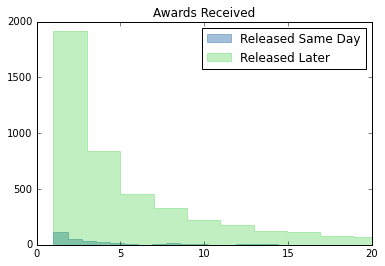
plt.hist(netflix_rel["Awards Received"], bins=150, histtype="stepfilled", color="steelblue", edgecolor="steelblue", alpha = 0.5, label="Released Same Day")
plt.hist(netflix_nonrel["Awards Received"], bins=150, histtype="stepfilled", color="limegreen", edgecolor="limegreen", alpha = 0.3,  label="Released Later")
plt.xlim(0,20)
plt.legend()
plt.title("Awards Received")

    Text(0.5, 1.0, 'Awards Received')

png

Findings

From the above analysis and graphs, same day releases tend to do slightly better in ratings metrics (IMDb, Roten Tomatoes, and Metacritic), but worse for awards. The overall distribution, however, looks similar for all metrics. Netflix clearly has more content that was released later than content that was released same day.

print(sp.stats.ttest_ind(netflix_rel["Awards Received"], netflix_nonrel["Awards Received"], nan_policy="omit"))
print(sp.stats.ttest_ind(netflix_rel["Metacritic Score"], netflix_nonrel["Metacritic Score"], nan_policy="omit"))
print(sp.stats.ttest_ind(netflix_rel["IMDb Score"], netflix_nonrel["IMDb Score"], nan_policy="omit"))

Ttest_indResult(statistic=-3.6479126235294426, pvalue=0.00026695722943390597)
Ttest_indResult(statistic=4.25895186332051, pvalue=2.100142994661915e-05)
Ttest_indResult(statistic=4.664152901062096, pvalue=3.1415989320023794e-06)

Are Netflix Movies or Series better?

Using the netflix_1, netflix_series, and netflix_movie tables, we will try to answer if movies or series are better on Netflix.

I will use pandas functionality to find values in this case.

ms_imdb = netflix_1.groupby("Series or Movie").agg({"IMDb Score": ["mean", "median", "min", "max"]}) 
ms_rt = netflix_1.groupby("Series or Movie").agg({"Rotten Tomatoes Score":  ["mean", "median", "min", "max"]})  
ms_mc = netflix_1.groupby("Series or Movie").agg({"Metacritic Score":  ["mean", "median", "min", "max"]})  
ms_awards_n = netflix_1.groupby("Series or Movie").agg({"Awards Nominated For":  ["mean", "median", "min", "max"]}) 
ms_awards_r = netflix_1.groupby("Series or Movie").agg({"Awards Received":  ["mean", "median", "min", "max"]})

ms_imdb.loc["Dif"] = ms_imdb.apply(lambda x:x["Movie"] - x["Series"])
ms_rt.loc["Dif"] = ms_rt.apply(lambda x:x["Movie"] - x["Series"])
ms_mc.loc["Dif"] = ms_mc.apply(lambda x:x["Movie"] - x["Series"])
ms_awards_n.loc["Dif"] = ms_awards_n.apply(lambda x:x["Movie"] - x["Series"])
ms_awards_r.loc["Dif"] = ms_awards_r.apply(lambda x:x["Movie"] - x["Series"])


print(ms_imdb)
print(ms_rt)
print(ms_mc)
print(ms_awards_n)
print(ms_awards_r)

                    IMDb Score                 
                          mean median  min  max
    Series or Movie                            
    Movie             6.752828    6.8  1.6  9.7
    Series            7.543188    7.5  2.7  9.5
    Dif              -0.790361   -0.7 -1.1  0.2
                    Rotten Tomatoes Score                   
                                     mean median  min    max
    Series or Movie                                         
    Movie                       64.608014   70.0  0.0  100.0
    Series                      67.551948   69.0  8.0  100.0
    Dif                         -2.943934    1.0 -8.0    0.0
                    Metacritic Score                    
                                mean median   min    max
    Series or Movie                                     
    Movie                  58.064766   59.0   6.0  100.0
    Series                 60.457831   61.0  24.0   93.0
    Dif                    -2.393065   -2.0 -18.0    7.0
                    Awards Nominated For                   
                                    mean median  min    max
    Series or Movie                                        
    Movie                      16.031134    6.0  1.0  355.0
    Series                     16.053586    5.0  1.0  386.0
    Dif                        -0.022452    1.0  0.0  -31.0
                    Awards Received                   
                               mean median  min    max
    Series or Movie                                   
    Movie                 10.060777    4.0  1.0  300.0
    Series                 8.330275    3.0  1.0  232.0
    Dif                    1.730502    1.0  0.0   68.0

Plotly Box Plots (see pdf link)

px.box(netflix_1, y=”IMDb Score”, color=”Series or Movie”)fig = px.box(netflix_1, y=[“Rotten Tomatoes Score”,”Metacritic Score”], color=”Series or Movie”) fig.update_layout(xaxis_title=”“)fig = px.box(netflix_1, y=[“Awards Nominated For”,”Awards Received”] , color=”Series or Movie”) fig.update_layout(yaxis=dict(range=[0,50]), xaxis_title=””)

Dash Interactive Plot (work in progress)

import dash import dash_core_components as dcc import dash_html_components as html from dash.dependencies import Input, Output

app = dash.Dash(name)

app.layout = html.Div([ html.P(“y-axis:”), dcc.RadioItems( id=”y-axis”, options=[{“value”:x, “label”:x} for x in [“IMDb Score”, “Rotten Tomatoes Score”, “Metacritic Score”, “Awards Nominated For”, “Awards Received”]], value=”IMDb Score”, labelStyle={“display”:”inline-block”} ), dcc.Graph(id=”box-plot”), ])

@app.callback( Output(“box-plot”, “figure”), [Input(“y-axis”, “value”)] )

def generate_chart(y): fig = px.box(netflix_1, x=”Series or Movie”, y=y) return fig

app.run_server(debug=True)

Findings

From the above analysis and graphs, Series tend to do better than Movies except in awards recieved.

Have Netflix offerings in the US gotten better over time?

print(sp.stats.describe(netflix_usa["IMDb Score"], nan_policy="omit"))
print(sp.stats.describe(netflix_usa["Rotten Tomatoes Score"], nan_policy="omit"))
print(sp.stats.describe(netflix_usa["Metacritic Score"], nan_policy="omit"))
print(sp.stats.describe(netflix_usa["Awards Nominated For"], nan_policy="omit"))
print(sp.stats.describe(netflix_usa["Awards Received"], nan_policy="omit"))

print(sp.stats.describe(netflix_int["IMDb Score"], nan_policy="omit"))
print(sp.stats.describe(netflix_int["Rotten Tomatoes Score"], nan_policy="omit"))
print(sp.stats.describe(netflix_int["Metacritic Score"], nan_policy="omit"))
print(sp.stats.describe(netflix_int["Awards Nominated For"], nan_policy="omit"))
print(sp.stats.describe(netflix_int["Awards Received"], nan_policy="omit"))

    DescribeResult(nobs=3427, minmax=(masked_array(data=3.1,
                 mask=False,
           fill_value=1e+20), masked_array(data=9.5,
                 mask=False,
           fill_value=1e+20)), mean=7.108987452582434, variance=0.7507656703036957, skewness=masked_array(data=-0.58494017,
                 mask=False,
           fill_value=1e+20), kurtosis=0.97092352948447)
    DescribeResult(nobs=1398, minmax=(masked_array(data=0.,
                 mask=False,
           fill_value=1e+20), masked_array(data=100.,
                 mask=False,
           fill_value=1e+20)), mean=70.29828326180258, variance=556.8193384966559, skewness=masked_array(data=-0.95555808,
                 mask=False,
           fill_value=1e+20), kurtosis=0.28785962243728)
    DescribeResult(nobs=889, minmax=(masked_array(data=11.,
                 mask=False,
           fill_value=1e+20), masked_array(data=99.,
                 mask=False,
           fill_value=1e+20)), mean=61.008998875140605, variance=263.16883784797176, skewness=masked_array(data=-0.34313274,
                 mask=False,
           fill_value=1e+20), kurtosis=-0.24167529977164692)
    DescribeResult(nobs=1998, minmax=(masked_array(data=1.,
                 mask=False,
           fill_value=1e+20), masked_array(data=386.,
                 mask=False,
           fill_value=1e+20)), mean=14.783783783783784, variance=1012.4720053052552, skewness=masked_array(data=5.06791624,
                 mask=False,
           fill_value=1e+20), kurtosis=33.043619260042334)
    DescribeResult(nobs=1560, minmax=(masked_array(data=1.,
                 mask=False,
           fill_value=1e+20), masked_array(data=251.,
                 mask=False,
           fill_value=1e+20)), mean=8.888461538461538, variance=338.11840430256086, skewness=masked_array(data=6.20063926,
                 mask=False,
           fill_value=1e+20), kurtosis=53.107288568802055)
    DescribeResult(nobs=5979, minmax=(masked_array(data=1.6,
                 mask=False,
           fill_value=1e+20), masked_array(data=9.7,
                 mask=False,
           fill_value=1e+20)), mean=6.867620003345041, variance=0.8224475129888926, skewness=masked_array(data=-0.67596619,
                 mask=False,
           fill_value=1e+20), kurtosis=1.4157715600612804)
    DescribeResult(nobs=4040, minmax=(masked_array(data=0.,
                 mask=False,
           fill_value=1e+20), masked_array(data=100.,
                 mask=False,
           fill_value=1e+20)), mean=62.74480198019802, variance=652.1841769847942, skewness=masked_array(data=-0.55751596,
                 mask=False,
           fill_value=1e+20), kurtosis=-0.6884438498993233)
    DescribeResult(nobs=3187, minmax=(masked_array(data=6.,
                 mask=False,
           fill_value=1e+20), masked_array(data=100.,
                 mask=False,
           fill_value=1e+20)), mean=57.294006903043616, variance=299.3984668963742, skewness=masked_array(data=-0.1170702,
                 mask=False,
           fill_value=1e+20), kurtosis=-0.49802215814851447)
    DescribeResult(nobs=4371, minmax=(masked_array(data=1.,
                 mask=False,
           fill_value=1e+20), masked_array(data=383.,
                 mask=False,
           fill_value=1e+20)), mean=16.600320292839168, variance=1048.573171522103, skewness=masked_array(data=4.90868371,
                 mask=False,
           fill_value=1e+20), kurtosis=31.481340395802768)
    DescribeResult(nobs=3659, minmax=(masked_array(data=1.,
                 mask=False,
           fill_value=1e+20), masked_array(data=300.,
                 mask=False,
           fill_value=1e+20)), mean=10.075157146761411, variance=396.3828135004485, skewness=masked_array(data=5.83951315,
                 mask=False,
           fill_value=1e+20), kurtosis=50.26291545901329)

Creating Time Series

netflix_usa_t = netflix_usa.groupby(pd.Grouper(key ="Netflix Release Date", axis=0, freq="1D", sort=True)).mean().dropna()
netflix_usa_t2 = netflix_usa.groupby(pd.Grouper(key ="Netflix Release Date", axis=0, freq="1D", sort=True)).mean().dropna()
netflix_index = pd.Series(np.array(range(1,224)))
netflix_usa_t2 = netflix_usa_t2.set_index(netflix_index)

Time Series Plots

px.line(netflix_usa_t, x=netflix_usa_t.index, y=”IMDb Score”)px.line(netflix_usa_t, x=netflix_usa_t.index, y=[“Rotten Tomatoes Score”,”Metacritic Score”])

Linear Regression of IMDb Score

imdb_x = np.array(netflix_usa_t2.index).reshape((-1,1))
imdb_y = np.array(netflix_usa_t2["IMDb Score"])
imdb_model = LinearRegression().fit(imdb_x, imdb_y)

imdb_model.score(imdb_x, imdb_y)
print("slope: ",imdb_model.coef_)
print("intercept: ", imdb_model.intercept_)

    slope:  [5.19102418e-05]
    intercept:  6.961315171694573

From the above results, we can see that the average Netflix offering in the US has not gotten better over time.